Matchup Methodology:

Prior to comparing satellite and in situ salinity data, these datasets with different spatiotemporal sampling (swath versus point) must be matched up. A detailed comparison of different matchup methods may be found in the matchup recommendation document​. Some different possibilities for matchup criteria include in situ centered vs. satellite centered;  time priority vs. space priority; single point matchup vs. multipoint average matchups. For validation purposes, an in situ centered matchup with “All-in-box” averaging over a 50km search radius and a ± 3.5-day time window produce the best results and are used here. A detailed, step by step description of matchup procedure implementation for L2 and L3 data is provided in the validation reports.  Matchups are then further quality controlled by applying two sets of data flags to the satellite observations, one which removes only the most heavily contaminated data and a second which applies all of the data flags to illustrate the best performance of satellite data.

For more details, please view our matchup recommendation document as well as our validation reports.


Illustration of likely mismatches when using a time‐centric approach to single sample difference matches. The ellipses indicate the 100x85km beam from Aquarius/SAC‐D for 10 – 1.44s integrations as it approaches an in situ measurement, denoted by a star. The first 1.44s integration that matches the criteria ΔT<±3.5 days and ΔS<50km, while minimizing ΔT is indicated by a blue ellipse. This is the single sample difference in time (SSDT) matchup. The green ellipse denotes a perfect match in space that occurs 7.2 s after this first match and would be chosen in a space‐centric approach. This is the single sample difference in space (SSDS) matchup. (from matchup recommendation document)

Example of Aquarius tracks near an Argo float (red arrow) in the Indian Ocean in 2011. Blue dots represent 1.44s integration times of Aquarius, while the red dot indicates an Argo observation. (from matchup recommendation document)


Triple Point Collocation:

Triple point collocation is a method to determine dataset errors when 3 independent datasets of the same variable are available. A benefit of triple point analysis over other error analysis methods is it does not require a priori assumption about which dataset is the “truth.” Rather, errors are determined for all datasets simultaneously. Triple collocation analysis is frequently used in the analysis of satellite errors. For current validation efforts, we use the covariance notation outlined in Stoffelen (1998) and Gruber et al. (2016) as it does not require datasets be scaled into a common dataspace. A detailed discussion of the underlying assumptions (signal error linearity, signal and error stationarity, error orthogonality, zero error cross-correlation, and dataset representativeness) can be found in Gruber et al. (2016).

The unscaled error variance (σε2) is:

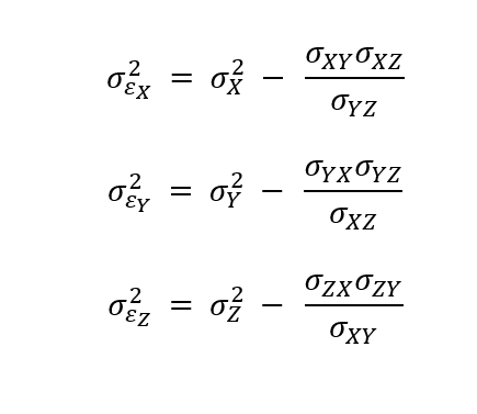
where, σi2 is the dataset variance and σij are the dataset covariances. The first term on the right-hand side represents the dataset variance, while the second term represents the sensitivity of the datasets. RMSD is √(σε2 )  for positive error variances. Errors are undefined if the sensitivity of the datasets is more than the dataset variance.

Generalized triple point collocation code and use case implementation in MATLAB and Python are located on ESR’s GitHub. https://github.com/EarthAndSpaceResearch/PiMEP

References

Gruber, A., Su, C. H., Zwieback, S., Crow, W., Dorigo, W., & Wagner, W. (2016), Recent Advances in (Soil Moisture) Triple Collocation Analysis. International Journal of Applied Earth Observation and Geoinformation, 45, 200-211.

Stoffelen, A. (1998), Toward the True Near‐Surface Wind Speed: Error Modeling and Calibration Using Triple Collocation. Journal of Geophysical Research: Oceans, 103(C4), 7755-7766.