

Funded by NASA
The OISSS dataset grids the Level-2 orbital data from the Aquarius/SAC-D satellite mission (25 August 2011 to 7 June 2015), the Soil Moisture Active Passive (SMAP) satellite mission (April 2015 – present) and the Soil Moisture and Ocean Salinity (SMOS) satellite mission (January 2011-present) onto a 0.25-degree spatial and 1-day temporal grid using Optimal Interpolation (OI).
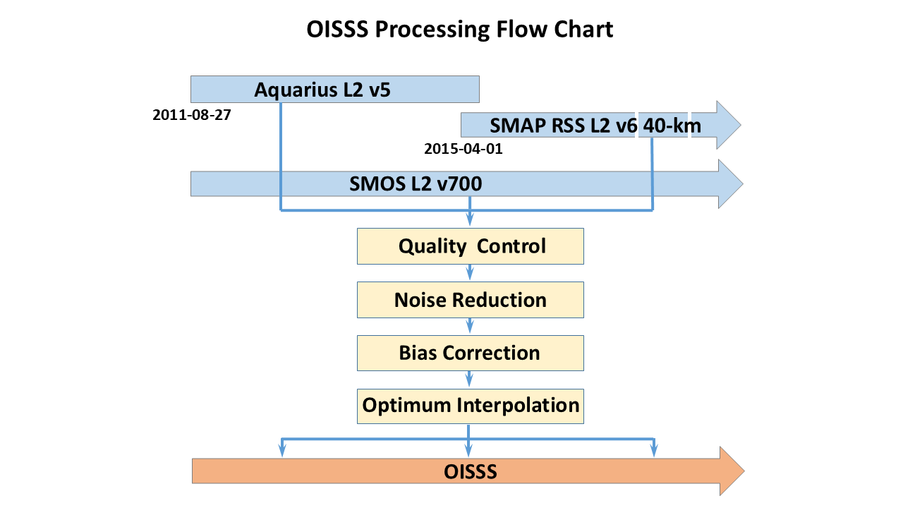
Input Data:
The input data are Level 2 SSS retrievals from the Aquarius, SMAP and SMOS satellites.
- Aquarius Level 2 (L2) version 5.0 (end-of-mission) data are produced by the NASA Goddard Space Flight Center’s Aquarius Data Processing System (ADPS) and distributed by the Physical Oceanography Distributed Active Archive Center (PO.DAAC) of the Jet Propulsion Laboratory (JPL), available at https://podaac.jpl.nasa.gov/dataset/AQUARIUS_L2_SSS_V5.
- SMAP observations of SSS are obtained from Level 2 version 6.0 SMAP data produced by the Remote Sensing Systems (RSS; www.remss.com).
- SMOS observations of SSS are obtained from the SMOS Level 2 SSS data products generated by version 700 of the Level 2 OS Operational Processor (L2OS). The data are available from the ESA SMOS online dissemination service at https://smos-diss.eo.esa.int/oads/access/.
Quality control:
Level 2 data from each of the three satellites are first processed to identify quality control (QC) issues. Quality control flags and auxiliary data (such as SST, surface wind, etc.) are used to eliminate questionable data points. Statistical tests based on the standard deviation (STD) are also applied to the data to remove outliers and reduce noise.
Noise reduction:
Additional noise-reduction algorithms are applied to mitigate high-frequency instrument noise. For Aquarius data, filtering is conducted along satellite tracks, whereas for SMAP and SMOS data, filtering is conducted in the temporal domain.
Bias correction:
Level 2 satellite data are adjusted to account for large-scale biases. Only static (time-mean) biases are considered. The bias fields are determined relative to in-situ salinity data.
Optimum Interpolation:
Bias-adjusted SSS retrievals are mapped onto a regular 0.25-degree, 4-day grid using a spatial Optimum Interpolation (OI) scheme (Bretherton et al., 1976). At each grid point, the SSS field is estimated via a weighted least-squares fit to the surrounding observations, where the weights are designed to minimize the estimation error variance. Subsequently, a temporal OI procedure is applied to the 4-day SSS fields to generate daily time series.
Output Data:
Multi-mission sea surface salinity optimum interpolation (OISSS) analysis. The OISSS dataset is available from 28 August 2011 to present.
A detailed description of the OISSS processing algorithm can be found in its user guide: OISSS_Product_Notes_v3.pdf
References
Bretherton, F. P., R.E Davis, and C.B. Fandry, 1976: A technique for objective analysis and design of oceanographic experiments applied to MODE-73, Deep Sea Res., 23, 559-582.
Melnichenko, O., P. Hacker, N. Maximenko, G. Lagerloef, and J. Potemra, 2014: Spatial Optimal Interpolation of Aquarius Sea Surface Salinity: Algorithms and Implementation in the North Atlantic, J. Atmos. Oceanic Technol., 31, 1583-1600.
Melnichenko, O., P. Hacker, N. Maximenko, G. Lagerloef, and J. Potemra, 2016: Optimum interpolation analysis of Aquarius sea surface salinity, J. Geophys. Res. Oceans, 121, 602-616, doi:10.1002/2015JC011343.